Checklist for Graphs
You must perform the following functions before you turn in any reports. These actions are easy to do and can immensely improve the professional character of your report (Show Me). Please check off the following and turn this form in with your report. Reports will not be accepted for grading until you have undergone these checks and may be considered as “late” if they must be returned to you for lack of your attention to these details.
Where possible and appropriate, I have presented multiple related curves on the same plot so that they can be readily compared. (How?)
I eliminated the gray background (How?)
I did not used the “smoothed curve” option. If there is no theoretical curve and no appropriate curve fit, I have not connected the symbols or have connected them with straight lines (How?).
I represented collected data with symbols, and theoretical curves with lines (How?).
I used line modes, line thicknesses or symbols to distinguish data sets, not colors (How?).
I eliminated gridlines from my plots (How?).
I made the numbers on the x and y axes large enough to read (How?).
I made the scales on the x and y axes follow the 1, 2, 5 rule (How?).
I labeled the x and y axes clearly with the information they represent and the correct units of the data (e.g. Frequency (Hz) or Pressure (dynes/cm2)) (How?).
I made the y-axis labels (title and numbers) run vertically from the bottom of the plot to the top, rather than horizontally (How?).
If Greek letters, other special characters, or superscripts/subscripts are needed in an axis title or elsewhere, I have used the capability of excel to include them (How?)
I made the legend for each curve descriptive of the curve (e.g. “cell growth with fibrinogen”, “cell growth without fibrinogen”, not “first data set”, “second data set”, and certainly not “series 1; series 2”) (How?).
I placed the legend on the plot area at a location where it does not cover any of the data. (How?)
Where applicable, the legends appear in an order that follows the position of the curve on the plot (i.e., upper curve matches the topmost legend) (How?).
I eliminated unnecessary borders, including:
a. The border around the legend.
b. The border around the plotting area.
c. The border around the complete plot. (How?)
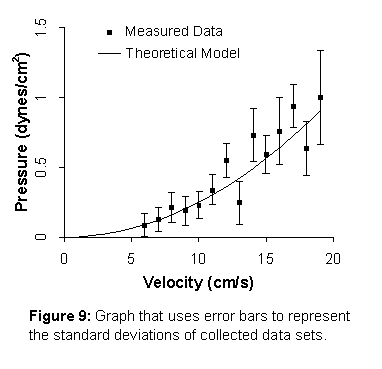
Where applicable, I have included bars representing standard deviation or standard error of my collected data (How?).
 Figures
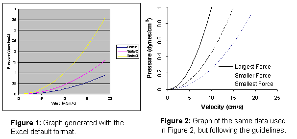
1 and 2 demonstrate the more professional look of a plot that follows the above
guidelines. Figure 1 uses the default
format of Excel. Figure 2 presents the
same data, but additional care has been taken to follow the guidelines.
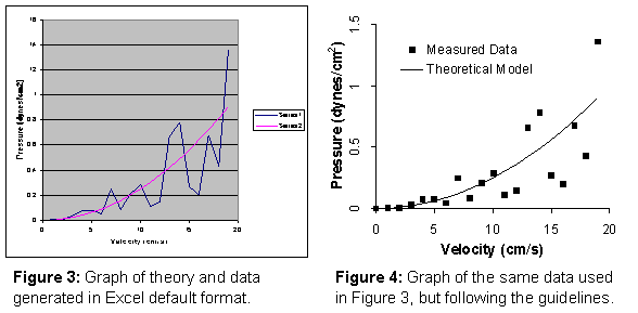
The example in Figures 3 and 4 shows a comparison between theoretical and experimental data formatted by default and then in a more professional style.
Excel generally attempts to determine how your data are ordered when you make a plot. For example, if you have 4 columns of data and you highlight all four columns, then click on the “Chart Wizard” toolbar and select “scatter plot,” Excel assumes that you wish to use the data in the first column for x-axis values and to use the other three columns as y-axis values for three separate curves. Sometimes you will need to manually tell Excel which data sets are to be used for x and y values on each curve.
To change the data you wish to plot, right click on the plot you have created and go to “Source data.” Select the “Series” tab. To change the x-axis values, click in the window labeled “X Values,” and then use the cursor to go back to your spreadsheet and highlight the data you wish to use. The “X Values” window will now display that range (e.g. “=sheet1!$A$1:$A$21”). Similarly, to change the y-axis values, click in the window labeled “Y Values,” and use the cursor to select the data values that you wish to use.
You can add additional data series by clicking on the “Add”
button on the lower left below the window labeled “Series.” Select the x and y data values as described
in the previous paragraph.
To remove the gray background on the plot area, right click on the plot area and select “Format Plot Area.” On the right side of the resulting dialogue box, under “Area” select the circle next to “None.”
The “Smoothed Curve” option connects data points with a “spline fit” of the data. This feature is almost never desirable in scientific writing because it can make the data appear to behave incorrectly (e.g. showing negative values for something that must be a positive quantity. To eliminate this option, right click on the data series in question, go to “format data series,” select the “Patterns” tab, and uncheck the box next to “Smoothed Curve” near the bottom left of the dialogue box.
Symbols and Theoretical Curves
To represent discrete data points with symbols, right click on the data series in question, go to “format data series,” select the “Patterns” tab, and left click on the arrow to the right of the box next to “Style.” You can select a “Foreground Color,” which is the color for the outline of the symbol and a “Background Color,” which is the color that will fill the inside of the symbol.
You can distinguish different data sets by different symbols and different fill options. For example, Squares vs. diamonds vs. triangles, or filled squares vs open squares. Be consistent in selecting symbols. For example, if you are plotting x vs y for two models at three different temperatures, you can make model 1 always be filled symbols and model 2 always be unfilled symbols and differentiate the temperatures as boxes, diamonds and triangles.
Whenever possible, it is best to generate plots in black and white rather than color. While colors may look nice, they do not necessarily copy well. While you may believe that it does not matter because you plan to print your final thesis in color, consider that your thesis committee will probably have a black and white copy of your work. In addition, if someone wishes to make a copy of your thesis, they will probably use black and white (which is still far cheaper than color printing) and may miss important aspects of your work. If you are making a plot for a presentation, remember that some colors do not appear at all when displayed on computer projectors, leading you to tell your audience, with great embarrassment, that “It looks fine on my computer screen.” You will then have to explain to them what the data set “would look like” if they could see it.
To change the character of plotted curves, right click on the data series in question, go to “format data series,” select the “Patterns” tab. To change the color of the line to black, left click on the arrow next to “Color” (which usually says “Automatic” by default) and select the black box. To change the line mode (solid, dashed, dotted) left click on the arrow next to “Style” and select the desired mode. To change the thickness of the line, left click on the arrow next to “Weight” and select the desired line thickness.
Note: If you are plotting a large number of points, the dashed and dotted line mode options will not work correctly. You can make it work correctly if you reduce the number of points in your data set (e.g., keeping only every 5th point). One simple way to do this is to highlight the data points that you want to keep (using CTRL+left-click), then use copy, and then past the results to another location in the spreadsheet.
By default, Excel plots have horizontal gridlines in them. These lines are generally distracting and should be removed. To do so, right click on the plot area and go to “Chart Options.” Then select the “Gridlines” tab and uncheck the box under “Value (y) axis” and next to “Major gridlines.”
To change the font size on an axis title, right click on the label and go to “Format Axis Title.” Then click on the Font tab and select the font size from the window under “Size” at right side of the dialogue box. The font size should be at least 12.
To change the font size on an axis numbers, right click on one of the numbers and go to “Format Axis.” Then click on the Font tab and select the font size from the window under “Size” at right side of the dialogue box. The font size should be at least 12.
The axes of graphs are most easily read if they are labeled in increments of 1, 2 or 5. (This scheme works well because we live in a base 10 society where we are familiar with breaking things up into 10 subunits and because 2 and 5 are the factors of 10). For example, if the data range from -13 to 17, a good label scheme would make the axis range from -15 to +20 with labels at -15, -10, -5, 0, 5, 10, 15, and 20 (increments by 5s). You generally do not want to have more than 7 labels on your plot, so an acceptable alternative would be to set a scale from -20 to +20 and have labels at -20, -10, 0, 10 and 20 (increments by 1s). Axes that are labeled in other increments (e.g. 3, 4, or 2.4032) are difficult to interpolate by eye.
To change the axis scale, right click on the numbers next to the axis and go to “Format axis.” Select the “Scale” tab and fill in appropriate values for “Minimum,” “Maximum,” and “Major unit.” E.g., for the first scaling in the paragraph above, Minimum would be -15, Maximum would be 20, and Major unit would be 5.
Related notes:
It is best to use units that yield number labels in the range of 0.1 to 1000, if possible. For example, if you are comparing cell diameters, use mm, do not use meters.
Avoid using exponential notation if possible.
Never assume that the physical quantity and dimensions of an axis are obvious. Even something as obvious as “Volts” might be plotted in millivolts or kilovolts. To provide a title for an axis (e.g. “Pressure (mm Hg)”, right click on the plot and go to “Chart options.” Select the “Titles” tab, and type the appropriate label in the box under either “Value (x) axis” or “Value (y) axis,” as appropriate. You can also create a graph title under this tab, although a title label is not always necessary since you will typically use other methods to create a figure caption.
Excel allows you to change the orientation of text. To do so, right click on the text, go to “Format axis” or “Format axis title” and hit the “Alignment” tab. Drag the text needle in the window on the right hand side of the dialogue box so that it has the orientation you need.
Greek Letters, Superscripts and Subscripts
Excel allows you to use Greek letters in the x and y axis titles. To take advantage of this feature, you should first type the axis title in its approximate form. For example, enter “dynes/cm2” as “dynes/cm2.” Now left click once on the legend to enter into an editing mode (for a vertical text y-axis, you will need to click twice slowly). In this mode, highlight the character or characters that you would like to change, and then right click on the highlighted text and go to “Format axis title.” Select the “Font” tab. To make the character(s) into superscripts or subscripts, check the appropriate box in the lower left portion of the dialogue box. To change a character into Greek, scroll down in the “Font” menu box until you find the “Symbol” font. When this font is selected, western characters are changed to Greek. For example, “a” is changed to “a,” and “D” is changed to “D.” Thus, you can enter “DP (dynes/cm2)” by first entering “DP (dynes/cm2)” and then changing the “D” to its Greek equivalent and changing the “2” to be a superscript.
Extra borders are unnecessary and generally distracting. They can also get into the way of important information. Compare, for example, the two plot styles shown in Figures 5 and 6. The data and other information are better emphasized when the following are eliminated:
a. The border around the legend (labeled “1” in Figure 5).
b. 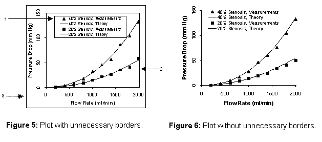 The
border around the plotting area (labeled “2” in Figure 5).
c. The border around the complete plot (labeled “3” in Figure 5).
To remove the boarder around the whole chart, right click on the region outside of the plot area, but inside the whole chart and go to “Format chart area.” Select the “Patterns” tab and click on the circle labeled “none” under the window on the left labeled “Border.”
To remove the border around the plotting area, right click inside the plotting area (but not on one of the curves or data symbols) and go to “Format plot area.” Select the “Patterns” tab, and click on the circle next to “none” under the window on the left labeled “Border.”
To remove the border around the legend, right click on the legend, and go to “Format legend.” Select the “Patterns” tab, and click on the circle next to “none” under the window on the left labeled “Border.”
To change the legends associated with each data set, right click on the plot and go to “Source data.” Select the “Series” tab, and click on the data set you are interested in changing in the window labeled “Series” in the lower left hand side of the dialogue box. (The data sets are usually labeled “series1, series2, series3, etc. by default). Then, in the window under “name” in the lower right hand side of the dialogue box enter the name you would like to associate with that data set. Once the name is entered, go back to the “Series” window to the left and click on any one of the series names. (You can also hit the Enter key, but this key will take you out of the “Source data” dialogue box instead of allowing you to change the name of another data set).
The best location for a plot legend is usually on the plotting area itself, but in a location that is away from any of the plotted data. To change the position of a legend, simply left click on the legend and drag it to the position you desire.
It is natural for a reader to assume that when several curves appear, the uppermost curve will correspond to the uppermost legend. An example of incorrect and correct legend positions is shown below:
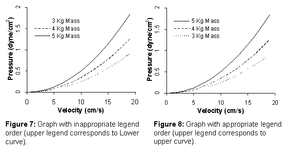
The order in which each series appears in the legend can be changed, although this feature is somewhat less intuitive than some of the others. To change the position of entries in the legend, right click on any one of the data curves and select “Format data series.” Select the “Series order” tab, and use the “Move up” and “Move down” buttons to move each legend to the desired position in the list.
Whenever repeated measurements are made at a given set of parameters, it will be important for the reader to know not only the mean value of each data point, but also the standard deviation or standard error, whichever is appropriate. To add error bars to a data set, right click on the data set and go to “Format data series.” Click on the desired error bar type (typically “Both” when you are plotting discrete points and “Plus” when you are using bar plots). You will usually want to select “Custom” in the lower left side of the dialogue box, which allows you to specify a different standard deviation for each data point. If you have calculated your standard deviations and placed them in a column of data, you can now click the cursor into the window labeled “+” and then highlight the column of standard deviations, which will fill in the dialogue box. Then click the cursor into the window labeled “-“ and again highlight the standard deviations column. Of course, you need to ensure that the standard deviations match the correct data point, which is why it is usually a good idea to keep your standard deviations in a column next to the mean values. An example plot with standard deviations is shown below.
