The Word 2007/2010 Equation Editor
Contents
The Word 2007/2010 Equation Editor 1
When the Equation Editor Should Be
Used. 1
Why the Equation Editor Should Be
Used. 1
How to Enter the Equation Editor
Quickly. 2
Equation Display Modes. 2
Equation Editor Options. 2
Math Autocorrect: A Useful Look-up
Tool 4
Insertion of Single Symbols. 5
Insertion of Spaces. 6
Grouping and Brackets. 7
Superscripts and Subscripts. 7
Division and Stacking. 7
Parentheses size control with
\phantom and \smash. 9
Square Roots and Higher Order Roots. 10
Integrals, Products and Sums. 10
Function Names. 10
Other Font Changes. 11
Accent Marks, Overbars, Underbars,
Above and Below.. 11
Greek Alphabet 12
Hebrew Characters. 12
Equation Numbers. 12
Symbol that Lack Keywords. 13
References. 14
The equation editor should be used to format your
equations. In some cases you can use simple Word commands, such as superscript
(<control>+) and subscript (<control>=) to format simple variables,
as when you wish to say, “L1 is the length of the beam,” but
in doing so, you should pay attention to the font in which the variable is
displayed. For example, variables should be formatted in italic font, while
function names and units of measure should be in regular font. (It is often
easiest to use a shortcut key, as described below, to jump into the equation
editor, even if you are simply typing a variable name).
Some equations will be nearly impossible to represent
without this editor. Others will simply look unprofessional. Compare the
following:
dy ax2 + bx + c
--- = --------------- sin(q)
dx (x – a)2
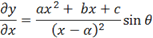
The second form looks better, requires about a third of the
time to create with the equation editor, and is far easier to modify. You can
save substantial time if you become familiar with the shortcut commands within
the equation editor. This document describes the use of the editor available
in Word 2007. This environment differs from the keystroke-based editor that
was available in previous versions of Word or in Mathtype. Its syntax is
similar to that of TeC a typesetting
program that pre-dates Microsoft Word.
The quickest way to enter the equation editor is the
shortcut key <alt>= (hold down the <alt> key while
you type “=”). You can also click on “Equation” under the “Insert” tab, but
this sequence can become cumbersome when you are setting a large number of
equations or defining multiple variables within text. The need to move your
hands from the keyboard to the mouse (or mouse pad) slows your typing.
You now have no excuse not to use the equation editor on a
casual basis. It is only one keystroke away.
While in the equation editor, you can use various symbols
and keywords instead of the more cumbersome menu bar. A more complete
description of the codes used by the equation editor and the syntax and
philosophy behind it is given by Sargent [1].
Single characters, such as _, ^ and /
that have special meanings.
Keywords such as \alpha that will be translated to
symbols (in this case,  ).
).
Keywords such as \sqrt and \overbrace will modify
expressions that are correctly grouped.
Note: Spaces that you type are important to the
equation editor because they tell the editor when it is time to translate a
part of the equation you are typing. Where it is necessary for clarity in this
document, a space will be represented by the sequence <sp>.
If you click on an equation, it will become highlighted, as
shown in Figure 1. When you then click
on the blue downarrow at the lower right, five options appear. “Save as new
equation…” allows you to keep the equation as a building block, which makes it
available from the “Insert” ribbon. “Professional” means that the equation
should be displayed as a formatted equation. “Linear” means to show the
equation in its raw form, similar to the way that the equation was typed, but
with some of the typed codes translated into special characters. “Display”
means that the equation will be formatted in a way that is appropriate for an
equation between paragraphs. “Inline” means that the equation will be
formatted in a way that is appropriate for an equation within a paragraph.
Inline equations tend to be more compressed than displayed equations.
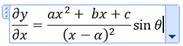
Figure 1: The appearance
of an equation.
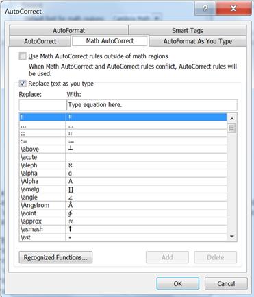
If you find that the equation editor does not format some
aspects of equations according to your taste, you may be able to change those
aspects with the Equation Options menu. To find this menu, enter the equation
editor (<alt>=), and when the “Design” ribbon appears, click on the arrow
(circled in red in Figure 2) at the
lower-right corner of the “Tools” group. This menu allows you to change, for
example, the default font for equations, the placement of integral limits, and
margins. It also is the gateway to the Math Autocorrect window discussed in
the next section.
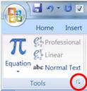
Figure 2: The tools
group of the Design ribbon.
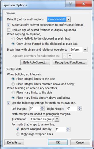
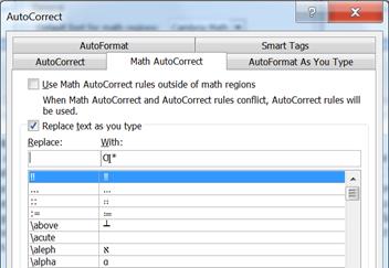
Figure 3: The Equation Options menu.
The equation editor causes brackets (such as [], {} and ( ))
to grow to the size of the expression within them. However, parentheses are
the grouping character and will not display when used as such. To force
parentheses to display, you must double them. To prevent brackets from being
reformatted, precede them by the “\” character. Some examples follow.
|
To Display
|
Type
|
Comments
|
|

|
[a/b]
|
The “/” command for fractions is described in a later
section.
|
|

|
{a/b}
|
|
|

|
(a/b)
|
Parentheses display.
|
|

|
a/(b+1)
|
Parentheses used for grouping do not display.
|
|

|
a/((b+1))
|
Double parentheses display.
|
|

|
{ a\atop b \close y
|
The \close keyword completes the opened brace.
The \atop command is described in a later section.
|
|

|
|(a|b|f)/(c+d)|
|
The parentheses are, again, used for grouping.
|
|

|
|a|b|f/(c+d)|
|
|
|

|
y=\[<sp>a/b<sp>\]
|
Backslashes prevent [ and ] from growing.
|
|

|
\norm a\norm
|
|
The _ and ^ keys are used to insert superscripts and
subscripts. Grouping is important because it distinguishes between  and
and  .
Terms can be grouped by enclosing them in parentheses, where the parentheses
themselves do not print. Some simple examples follow:
.
Terms can be grouped by enclosing them in parentheses, where the parentheses
themselves do not print. Some simple examples follow:
|
To Display
|
Type
|
Notes
|
|

|
x_i\times<sp>y^n
|
The spacebar <sp> is needed.
|
|

|
x^(i+1)
|
The parentheses do not show. See “grouping.”
|
|

|
x_i^n
|
|
|

|
F_n^(k+1)
|
|
|

|
F_(n^(k+1))
|
All of the parentheses are needed.
|
|

|
(_0^9)H
|
|
Use the “/” character for
division. The equation editor will reformat the expression to place the
numerator above the denominator. To prevent vertical buildup of the fraction,
use “\/” instead of “/” alone. As with superscripts and subscripts, you can use
parentheses to group expressions into a numerator and denominator. Examples
follow:
|
To Display
|
Type
|
Comments
|
|

|
a/b
|
|
|

|
(a+b)/(c+d)
|
Parentheses do not print.
|
|

|
((a+b))/(c+d)
|
The double parentheses force the single parentheses to print
in the numerator.
|
|

|
((a+b)/(c+d) +
n)/(f(x)+e^(1\/2))<sp>
|
The “/” is preceded by “\” in the exponential to provide a
horizontal fraction ( instead
of instead
of  ). ).
|
If you need to stack expressions without the horizontal
division line, use \atop or \matrix. The vertical bar “|” can also be used in
place of \atop.
|
To Display
|
Type
|
Comments
|
|

|
a\atop b or a|b
|
Do not add spaces between the expression and the vertical
bar.
|
|

|
(a+b)\atop(c+d)
|
Parentheses do not print.
|
|
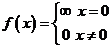
|
f(x)={\matrix (\infty x=0@0 x\ne 0) \close
|
The @ character ends a row of the matrix.
|
|
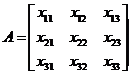
|
A=[\matrix(x_11&x_12&x_13@
x_21&x_22&x23@
x_31&x_32&x_33)]
|
The matrix must be enclosed in ()’s. The & character
separates columns of the matrix. The @ separates rows.
|
The syntax for matrices tends to lead to expressions that
are difficult to read. An easier approach is to enter the equation editor with
<alt>+ and then use the Matrix dropdown menu in the structures group to
insert the closest approximation to the matrix that you need. To add extra
columns and rows, click on the equation and then click on the small blue
down-arrow and scroll down to “Linear” to change the display to linear, then
insert “&” and “@” symbols as appropriate, and return to “Professional.”
The keywords \phantom and \smash can be used to force brackets
and parentheses to have a specific size.
|
To Display
|
Type
|
Comments
|
|

|
[\phantom (a\atop b)]<sp>
|
The \phantom command creates an object as large as the
expression in parentheses, but does not print it, so you can create, for
example, large empty brackets.
|
|

|
[\smash(a\atop
b)\close<sp><sp>
|
\smash creates the object, but makes its size zero so that
the enclosing bracket does not grow.
|
|

|
[\hphantom((a+b)/c)]
|
The \hphantom command creates an object with the width of
the expression in parentheses, but zero height.
|
|

|
[\vphantom((a+b)/c)]
|
The \vphantom command creates an object with the height of
the expression in parentheses, but zero width.
|
This example shows a Routh matrix that was constructed with
the aid of “\vphantom.”
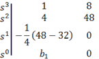
Without the \vphantom, the vertical spacing of the stack of  symbols
on the left would not match with that of the two columns on the right.
symbols
on the left would not match with that of the two columns on the right.
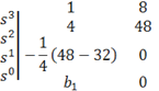
The syntax is
\open\matrix(s^3@s^2@⇳(1/4)
s^1@s^0 )| \matrix(1&8\vphantom(s^3
)@4&48\vphantom(s^2
)@-1/4 (48-32)&0@b_1&0\vphantom(s^0
))
Yes. I do realize that this example is far more than you
want to worry about.
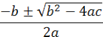
The square root keyword \sqrt operates on the argument that
follows it. The equation editor also has keywords for higher order roots.
Examples are:
|
To Display
|
Type
|
Comments
|
|

|
\sqrt x
|
|
|

|
\sqrt(x+1)
|
|
|

|
\cbrt(x+1)
|
|
|

|
\qdrt(x+1)
|
|
|
|
(-b\pm\sqrt(b^2-4ac))/2a<sp>
|
|
|

|
\sqrt(n&x)<sp>
|
The & separates the root order from the argument
|
Integrals, products and sums are inserted with the keywords
\sum, \int and \prod. Use subscripts and superscripts to insert the limits.
Examples are:
|
To Display
|
Type
|
|

|
\sum_(n=0)^N x^n<sp>
|
|

|
\prod_(n=0)^N x^n<sp>
|
|

|
\int_-\infty^\infty <sp> <sp> f(t) e^-i\omega
t<sp>dt
|
|

|
\iint f(x) dx
|
|

|
\iiint f(x) dx
|
|

|
\oint f(x,y) dl
|
The equation editor switches between “variable style” or
“function style,” depending on whether it interprets part of an equation as a
variable or a function (compare the two styles in the equation  , which
would not look right if it were displayed as
, which
would not look right if it were displayed as  ). You
must type a space after the function name to allow the editor to interpret it
as a function. Some of the functions that are recognized are:
). You
must type a space after the function name to allow the editor to interpret it
as a function. Some of the functions that are recognized are:
If a function keyword is not recognized, you can force the
editor to treat it as a function if you follow it with the \funcapply keyword.
For example,  is not
recognized as a function, but the sequence sinc\funcapply<sp><sp>
will produce
is not
recognized as a function, but the sequence sinc\funcapply<sp><sp>
will produce  (as
opposed to the less attractive
(as
opposed to the less attractive  .
.
Many of the utilities on the Font group of the Home ribbon
can be used to modify text within an equation. The \scriptX command (where X
is any single letter) can also be used to quickly create a script letter. For
example \scriptL produces  .
Similarly, \doubleL produces
.
Similarly, \doubleL produces  , and
\frakturL produces
, and
\frakturL produces  . The
size of an equation can be increased with the shortcut <control>] and
decreased with <control>[. The variable style can be overridden with
several commands. See Gardner [2] for more information.
. The
size of an equation can be increased with the shortcut <control>] and
decreased with <control>[. The variable style can be overridden with
several commands. See Gardner [2] for more information.
To Insert Use
a script character (e.g.  ) \scriptF
(Notice that there is no space between \script and F)
) \scriptF
(Notice that there is no space between \script and F)
regular text Enclose in
quotes. E.g. “a”= “b” produces  instead
of
instead
of  .
.
italic text toggle italic
on and off with <control>i
bold text toggle bold on
and off with <control>b
hello there <control>i
hello <control>I there
hello there <control>i
hello <control>b there
 \scriptL
{f(x)}
\scriptL
{f(x)}
 x=\Re(x+iy)
 y=\Im(x+iy)
|
a large character 
|
Select the character. Then, on the Design ribbon, under
the “Tools” group, click on “Normal Text.” Now go to the “Home” ribbon and
change the font size. Go back to the Design ribbon and click on “Normal
Text” again to get back to the correct font design (e.g. italic if it is a variable).*
|
* Sorry about this level of complication. There
should just be a command like \size24 to change the point size, but there is
not. Also, if you try to change font size without first clicking on “Normal
Text,” the font size of the entire equation changes, rather than just the
characters you selected.
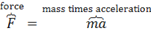
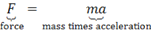
Certain keywords can be used to place accents, overbars,
overbraces and other modifiers on characters and expressions. Examples are:
|
To Display
|
Type
|
Comments
|
|
|
\overbrace<sp>F^”force” = \overbrace(ma)^”mass times
acceleration”<sp>
|
Overbrace text is introduced with ^, as if it were a
superscript.
|
|
|
\underbrace<sp>F^”force” = \underbrace(ma)^”mass
times acceleration”<sp>
|
Underbrace text is introduced with _, as if it were a
subscript.
|
|

|
\overbar(a+b)
|
|
|

|
\overparen(a+b)
|
|
|

|
\underbar(a+b)
|
|
|

|
lim<sp>_(x\rightarrow
0)<sp>f(x)
|
You can replace “_” with
“\below”.
|
|
|
lim<sp>\below(x\rightarrow
0)<sp>f(x)
|
Because “lim” is a keyword it is not displayed in italics.
|
|

|
lim<sp>\above(x\rightarrow 0)<sp>f(x)
|
Some accents are designed to fit over a single character.
The keyword must be typed after the modified character and followed by two
spaces.
|
For
|
Type
|
For
|
Type
|
For
|
Type
|
|

|
x\bar<sp><sp>
|

|
x\ddot<sp><sp>
|

|
x\hvec<sp><sp>
|
|

|
x\Bar<sp><sp>
|

|
x\hat<sp><sp>
|

|
x\tvec<sp><sp>
|
|

|
x\check<sp><sp>
|

|
x\tilde<sp><sp>
|
|
|
|

|
x\dot<sp><sp>
|

|
x\vec<sp><sp>
|
|
|
Prime marks also follow the expression that they modify, but
are followed by only a single space:
|
To Display
|
Type
|
|

|
x\prime<sp>
|
|

|
x\pprime<sp>
|
|

|
x\ppprime<sp>
|
To include a Greek letter in an equation, spell the name of
the letter, preceded by the backslash character (\). If the name begins with a
lower case letter, a lower case Greek letter is inserted. If the name begins
with an upper case letter, an upper case Greek letter is inserted. The table
below provides the names for each of the lower case Greek letters (with some
variations).
|
For
|
Type
|
For
|
Type
|
For
|
Type
|
For
|
Type
|
|

|
\alpha
|

|
\eta
|

|
\omicron*
|

|
\upsilon
|
|

|
\beta
|

|
\iota
|

|
\pi
|

|
\varpi
|
|

|
\chi
|

|
\varphi
|

|
\theta
|

|
\omega
|
|

|
\delta
|

|
\kappa
|

|
\vartheta
|

|
\xi
|
|

|
\epsilon
|

|
\lambda
|

|
\rho
|

|
\psi
|
|

|
\phi
|

|
\mu
|

|
\sigma
|

|
\zeta
|
|

|
\gamma
|

|
\nu
|

|
\tau
|
|
|
*\omicron should work,
but did not when I tried it in the Word 2007 editor. If you have trouble with
this letter, you can use the Symbols group of the Insert ribbon.
The equation editor’s collection of Hebrew characters is
limited to the first four.
 \aleph
 \beth
\beth
 \daleth
 \gimel
The easiest way to number
equations is to put the equation in a table. If you wish to have the equation
centered, use a table with three columns so that the left column balances the
right column. Here is an example. The table borders are included for clarity,
but in most cases, it is best to remove them.
|
|

|
Eq. 1
|
You can make the equations
automatically numbered if you click inside the table, go to the “References”
ribbon, and click on “Insert Caption.” Choose “Equation,” and use the label
that fits your taste (in this case, I have used “Eq.”). Finally, change the
“borders and shading” for the table to “None.”
To generate additional
numbered equations, you can copy and paste the table that you just generated into
different locations and simply change the equation. Highlight the equation
number, right click, and select “Update Field” to have Word automatically
change the number. To simplify matters further, you can just copy and paste
the above table into your document and use it as a template.
|
|

|
Eq. 2
|
The equation editor lacks
keywords for some symbols. Some missing keywords are surprising, such as one
for  , which
one would expect to be simply \Angstrom.
If the keyword cannot be found, the symbol is probably still available. First,
check the Symbols group on the Design ribbon under Equation Tools (Figure 5), which should appear when you type
<control>+ to enter the equation editor.
, which
one would expect to be simply \Angstrom.
If the keyword cannot be found, the symbol is probably still available. First,
check the Symbols group on the Design ribbon under Equation Tools (Figure 5), which should appear when you type
<control>+ to enter the equation editor.
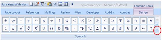
Figure 5: The Symbols
group under the Design tab of “Equation Tools.”
Most of the default symbols in
this group have already been described. However, if you click on the down-arrow
(circled in Figure 5) and then click on
the down-arrow at the top of the resulting menu, the following options will
appear:
Basic Math
Greek Letters
Letter-Like
Symbols
Operators
Arrows
Negated
Relationships
Scripts
Geometry
For example, the “Letter-Like Symbols” group contains the
following symbols, some of which do not have keywords.
|
Symbol
|
Name
|
ASCII Hexadecimal Code
|
|

|
Latin Small Letter Eth
|
00F0
|
|

|
Turned Capital F
|
2132
|
|

|
Hilbert Space
|
210C
|
|

|
The Set of Natural Numbers
|
2115
|
|

|
Rational Numbers
|
211A
|
|

|
Real Numbers
|
211D
|
|

|
The Set of Integers
|
2124
|
|

|
Angstrom
|
212B
|
|

|
Inverted Ohm Sign
|
2127
|
|

|
There Does Not Exist
|
2204
|
The ASCII hexadecimal code may be useful for a small subset
of people. If you type that code into an equation, then select the code and
type <alt>x (think of the “x” as standing for hexadecimal), it will
convert the number to the corresponding character. You can convert only one
character at a time. If you need to use an undefined symbol frequently, you
should create your own definition with the Math Autocorrect function described
in the section Math Autocorrect: A Useful Look-up Tool.
Conversely, if you are in the linear mode of the equation
editor, you can highlight a single character and then type <alt>x to print
that character’s hexadecimal code.
As a last resort, you can resort to using Symbol under the
Symbols group of the standard Insert ribbon, which is completely independent of
the equation editor.
1. Sargent, M
III, “Unicode nearly plain-tex encoding of mathematics,” Office Authoring
Services, Microsoft Corporation, 2006 (http://unicode.org/notes/tn28/UTN28-PlainTextMath-v2.pdf).
2. Gardner J,
“Shortcuts for the Word 2007 equation editor,” (http://dataninja.files.wordpress.com/2007/09/word07shortcuts.pdf).