Measurement Error
Assume that you have an
expression that relates a design criterion to the individual components of your
system.
Eq. 1
![]()
As a simple example, z could
be the gain of an amplifier, and w, x and y could be the values of three
resistors in an operational amplifier circuit.
Alternatively, z could be the peak sustainable force of a bone plate,
and w, x, and y could be the thickness, width and elastic modulus of the plate.
What is the anticipated
standard deviation of z, given the
tolerances in w, x and y? To answer this, we need a definition for
standard deviation. This definition is
given by:
Eq. 2
![]()
In other words, say that we
make N realizations of our
system. Then zi represents all of the values of z that we get in the N
prototypes, and ![]() represents the average
value of z, which should be the
design value.
represents the average
value of z, which should be the
design value.
Example
You are designing an
amplifier whose gain, A, depends on
the values of two resistors and a capacitor.
Your design value for A is 10,
which corresponds to ![]() . You make five
realizations, and their gains (
. You make five
realizations, and their gains (![]() ) come out to be 10.2, 10.3, 9.9, 10.5, and 9.4. The error in z,
) come out to be 10.2, 10.3, 9.9, 10.5, and 9.4. The error in z, ![]() , is:
, is:
Eq. 3
![]()
which has a value of 0.1875.
Relating Error in z to Component Errors
You know that z is related to the specific parameters
(w, x, y) through some
formula:
Eq. 4
![]()
We can expand this in a
Taylor series around the design value ![]() :
:
Eq. 5
![]()
where ![]() . Now substitute
Equation 5 into Equation 2.
. Now substitute
Equation 5 into Equation 2.
Eq. 6

The two terms, ![]() , cancel so that the result is:
, cancel so that the result is:
Eq. 7

There are two types of terms
in the summation. Three of them have the
form:

All of these are positive
valued and will add to the error in z.
There are also three “cross terms” of the form:
![]()
On average, half of these
terms will be positive and half will be negative (i.e. half of the time ![]() and
and ![]() will have the same
sign and the other half of the time they will have opposite signs). Consequently, these terms will tend to cancel
one another out, so that these cross terms will disappear when the summation is
taken. As a result, Equation 7 can be
rewritten as:
will have the same
sign and the other half of the time they will have opposite signs). Consequently, these terms will tend to cancel
one another out, so that these cross terms will disappear when the summation is
taken. As a result, Equation 7 can be
rewritten as:
Eq. 8

The summation can be taken
individually over each term. Since the
terms ![]() are the same for each
value of i, they can be brought out
of the summation to yield.
are the same for each
value of i, they can be brought out
of the summation to yield.
Eq. 9
![]()
But the definition of
standard deviation was defined in Equation 2:
![]()
So Equation 8 becomes the
equation in the book.
 Example
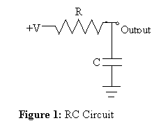
For the circuit shown in
Figure 1, the expression for gain is:
![]()
The derivatives with respect
to R and C are:
 ,
, 
Given values for ![]() and
and ![]() (standard deviations
for the resistance and capacitance, which are the tolerances coded onto the
elements), the error in A can be calculated as:
(standard deviations
for the resistance and capacitance, which are the tolerances coded onto the
elements), the error in A can be calculated as:

 From
this, the expected error in the gain, A,
can be calculated for any frequency
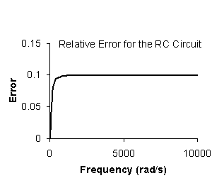
 ![]() . The result is shown
in Figure 2, assuming a 10% error in both the resistor and the capacitor. Recall that this is an estimate of the error. The
true error may be somewhat larger or somewhat smaller than what is shown,
depending on what the actual values of the resistor and capacitor are. It should not be surprising that the error
goes to zero as frequency goes to zero because for an RC circuit, regardless of
the resistor and capacitor values, the gain is 1 at frequency zero. As frequency increases beyond the 3 db point
(in this case
. The result is shown
in Figure 2, assuming a 10% error in both the resistor and the capacitor. Recall that this is an estimate of the error. The
true error may be somewhat larger or somewhat smaller than what is shown,
depending on what the actual values of the resistor and capacitor are. It should not be surprising that the error
goes to zero as frequency goes to zero because for an RC circuit, regardless of
the resistor and capacitor values, the gain is 1 at frequency zero. As frequency increases beyond the 3 db point
(in this case ![]() =100), the gain tends toward
=100), the gain tends toward ![]() , which explains why 10% error in the components leads to 10%
error in A.
, which explains why 10% error in the components leads to 10%
error in A.
Figure 2:
Relative error for the RC circuit, assuming an error of 10% in both the
resistor and the capacitor. The
resistor value is 10 KW. The capacitor value is 1 mF.
Exercise: For a circuit
that consists of three resistors in series (R1, R2 and R3),
where R2 and R3 have 10% variances and R1 has
a 5% variance, what is the variance in the equivalent resistance of the circuit
(Req = R1 + R2 + R3).
Steven A. Jones
BIEN 402, Biomedical Senior Design I
