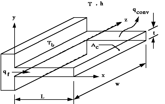
Figure 1. Rectangular Fin
LAB 5 - One-Dimensional Fin Heat Transfer
Introduction
A fin is an extended surface that is used specifically to enhance the heat transfer rate between a solid and an adjoining fluid. There are several different general fin configurations, including straight fins, which are extended surfaces attached to plane walls and annular fins that are circumferentially attached to a cylinder. These fin types may have rectangular cross sections, whose area may be expressed as a product of the fin thickness t and the width w for straight fins or the circumference for annular fins.
As previously indicated, the primary interest when analyzing fin performance is a determination of the enhancement of heat dissipation from a surface to the surrounding fluid. In order to determine the heat transfer rate from a fin, the temperature distribution along the fin must first be determined. The temperature distribution may be determined analytically if several simplifying assumptions are made. One-dimensional heat transfer in the longitudinal (x) direction is typically assumed, even though heat conduction within the fin is two-dimensional. The rate at which energy is convected to the surroundings from any point on the fin must be equivalent to the heat conducted to that point in the transverse (y, z) direction. However, since most fins are thin, the temperature changes in the x-direction are much greater than those in the transverse directions. Therefore, the temperature gradients in the y and z directions may be assumed to be negligible, and the analysis becomes one-dimensional. Additional assumptions include: steady state conditions, constant thermal conductivity, negligible radiation from the surface, no heat generation within the fin, and that the convection heat transfer coefficient h is uniform over the entire surface. With these assumptions, an application of the conservation of energy principle to the straight fin of uniform cross section, shown in Figure 1, will result in an ordinary differential equation that can be solved for the temperature in the fin.

Figure 1. Rectangular Fin
The fin temperature at the base is T(0) = Tb
while the surrounding fluid is at T![]() .
The rectangular fin has a uniform cross sectional area Ac
= wt. With these physical characteristics specified, the governing differential
equation is
.
The rectangular fin has a uniform cross sectional area Ac
= wt. With these physical characteristics specified, the governing differential
equation is

In order to simplify this equation, the dependent variable T may be
transformed by defining an excess temperature ![]() as
as
(2)
Since T![]() is a constant, d
is a constant, d![]() /dx
= dT/dx, and equation 1 can now be written as
/dx
= dT/dx, and equation 1 can now be written as

where

Equation 3 is a linear, homogeneous, second-order differential equation with constant coefficients. The general solution has the form
(5)
Boundary conditions must be utilized in order to determine the constants C1 and C2 in equation 5. One of the boundary conditions is a specified temperature at the base of the fin (x = 0).
(6)
A second boundary condition results from the convection heat transfer from the fin tip. An energy balance applied to a control surface about the tip indicates that the conduction to the tip must equal the heat transferred by convection from the tip to the surroundings.

Equation 7 may be restated in terms of the excess temperature,

Substituting the general solution, equation 5, into the boundary conditions, equations 6 and 8, gives the following
(9)
(10)
Equations 9 and 10 may be solved for C1 and C2. With the constants known, they may be substituted into the general solution, which, after some tedious algebra, results in

This equation expresses the temperature of the fin as a function of the longitudinal location. A typical temperature profile is shown schematically in Figure 2. With the temperature in the fin determined, it is now possible to calculate the total heat loss from the fin. Note that the heat transferred into the fin at the base equals the heat loss from the fin. Fourier's law applied at the base gives

With the temperature distribution known, qf can then be evaluated, giving

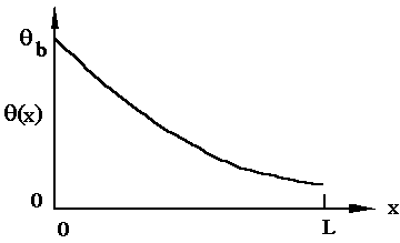
Figure 2. Temperature Profile in the Rectangular Fin
Determination of the Heat Transfer Coefficient
The heat transfer from a rectangular fin can be determine by several means. An experimental measurement of the heat entering the fin through the base could be used to determine the fin heat transfer. Alternately, equation 13 could be used, assuming the heat transfer coefficient is a known quantity. Unfortunately, h is the most difficult of the parameters in the equation to determine and is usually an unknown. Fortunately, a statistical method is available that utilizes experimental data representing the temperature profile in the fin to determine the value of the heat transfer coefficient.
The method of least squares is a statistical method that can be used
in this case to curvefit the experimental data. The data represents the
longitudinal position (x) and the corresponding temperature (T or ![]() )
at that position. Based upon the assumption that the errors in the experimental
measurements follow a Gaussian distribution, the method of least squares
produces a unique value for the constants to be determined. In other words,
the value of the constants determine the best fit of the data, given the
most probable form of the governing equation (the form of the curvefit
equation).
)
at that position. Based upon the assumption that the errors in the experimental
measurements follow a Gaussian distribution, the method of least squares
produces a unique value for the constants to be determined. In other words,
the value of the constants determine the best fit of the data, given the
most probable form of the governing equation (the form of the curvefit
equation).
The form of the curvefit equation for ![]() (x)
can be extracted from the analytical solution (equation 11). The proposed
curvefit equation is
(x)
can be extracted from the analytical solution (equation 11). The proposed
curvefit equation is

where the values of the constants A and B could be determined from equation 11 as


However, the values of A and B may also be found using the method of least squares. The strategy for fitting the "best" line through the data would be to minimize the sum of the squares of the residual errors Sr for all of the available data. The residual, or error, is the discrepancy between the measured data and the approximate value predicted by the curvefit equation. The residual for each set of data (ei) in this case can be expressed as

Then the sum of the squares of the residuals can be expressed as

In order to determine values for A and B, the residual must be minimized. Equation 16 is first differentiated with respect to each coefficient and the results are then set equal to zero.


These equations represent a set of 2 equations with 2 unknowns, A and B. The equations may be solved (with some difficulty) to give


Note that the denominator is the same in each equation and that the summation symbols have been simplified; all summations are from i = 1 to n. These equations may be designated as equations 19 and 20. Only one problem remains; the solutions for A and B are dependent upon the variable m, which contains the heat transfer coefficient h (the desired solution)! This dilemma may be overcome by an iterative procedure which will provide the best values of A, B, and h.
The best fit from the method of least squares may be provided by minimizing the variance, a statistical parameter that indicates the spread of the data about the curvefit line. The variance (Syx2) for this equation form is

Two possibilities present themselves for completing the iteration process. In order to find the minimum variance, the derivative of the variance with respect to m must equal zero. This requirement must be met in order to complete the iterative scheme. A second, less elegant solution method, involves the determination of the variance for a number of assumed values of h. The variance as a function of h is then plotted and the minimum inflection point on the graph will indicate the value of h for the fin. Figure 3 is an example plot of a possible functional relationship between the variance and h.
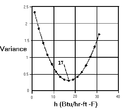
Figure 3. Example of Variance as a Function of Heat Transfer Coefficient
Objectives
This experiment was designed to demonstrate the concept of a fin as it relates to the heat transfer field and to present a statistical method for the determination of a physical parameter such as the heat transfer coefficient. Experience will also be gained in modeling the physical situation, in the acquisition of data that characterizes that physical situation (and the judicious use of same), and in the study of a one-dimensional approximation.
Experimental Apparatus
A model of a one-dimensional fin is provided for this experiment. Figure 4 details the fin dimensions and the approximate locations of the type K thermocouples while Table 1 gives exact thermocouple locations within the 304 stainless steel. In the present configuration, the fin is insulated on the bottom and sides with two inches of calcium silicate brick insulation. Thus, from a thermal point of view, the design represents the upper half of a symmetric, infinitely wide (in the z direction) fin.
Heat is supplied to the fin base by two Watlow strip heaters that are wired in parallel to a power supply. The maximum design total heat input is 600 watts. The thermocouples are connected to a 20 channel selector which, in turn, is connected to a digital readout.
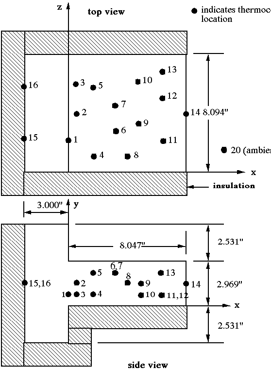
Figure 4. One-Dimensional Fin Dimensions
Table 1. Thermocouple Locations
|
|
|
|
|
|
|
|
|
|
|
|
|
|
|
|
|
|
|
|
|
|
|
|
|
|
|
|
|
|
|
|
|
|
|
|
|
|
|
|
|
|
|
|
|
|
|
|
|
|
|
|
|
|
|
|
|
|
|
|
|
|
|
|
|
|
|
|
|
|
|
|
|
|
|
|
|
|
|
|
|
|
|
|
|
|
|
|
|
|
Procedure
The apparatus will be turned on before class to ensure that a steady state condition exists. Do not touch any of the stainless steel surfaces or adjust the settings on the power supply.
In the discussion of the results the following items should be considered (as a minimum):