ME 354 - Thermofluids
Laboratory
Spring 1998
LAB 8 - Velocity Profile above a Flat Plate
Introduction
In any viscous flow, the fluid in direct contact with a solid boundary has
the same velocity as the boundary itself and the "no-slip condition" must
be satisfied at the boundary. Since the fluid velocity at the stationary
solid surface is zero, but the bulk fluid is moving, velocity gradients (and
hence shear stress) must be present in the flow. For one-dimensional viscous
flow, the shear stress t is given by
 (1)
(1)
where  = dynamic viscosity, u = stream wise velocity,
and y = normal coordinate measured from the solid
boundary.
= dynamic viscosity, u = stream wise velocity,
and y = normal coordinate measured from the solid
boundary.
Thus, for external flow over a flat plate as shown in Figure 1, the wall
shear stress can be determined from knowledge of the velocity profile.
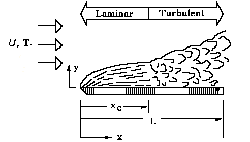
Figure 1. Flat Plate Boundary Layer
For an external flow in which the fluid is unbounded by walls, the viscous
effects will grow and continually expand as flow moves further downstream
along the solid surface. The viscous layers, either laminar or turbulent,
are very thin, much thinner than the drawing above shows. The boundary
layer thickness is defined as the point where the velocity u parallel
to the plate reaches 99% of the external free stream velocity U.
The accepted formulas of for
flat-plate flow are [1]
for
flat-plate flow are [1]
/x  5.0/Rex1/2 for laminar
flow (2)
5.0/Rex1/2 for laminar
flow (2)
In turbulent flow, the boundary layers expands more rapidly and the accepted
correlation for is
/x  0.16/Rex1/7
for turbulent flow
(3)
0.16/Rex1/7
for turbulent flow
(3)
A dimensionless quantity of particular interest in external flows is
cf, called the skin-friction coefficient, and is analogous to
the friction factor f in internal flows. cf is defined by
cf
= 2 /
/ U2
(4)
U2
(4)
where U = the free stream velocity outside the boundary layer,
= the shear stress
at the wall, and =
the density of the fluid.
Boundary layer theory, first formulated by Ludwig Prandtl in 1904, is one
method for obtaining solutions for laminar flow inside a boundary layer.
By making certain order of magnitude assumptions the Navier-Stokes
equations can be simplified into the boundary layer equations that may be
solved relatively easily in some simple geometries. Equation 3, Blassius's
solution is a result of a boundary layer solution. Blassius's
solution results in an ordinary differential equation that must be numerically
integrated. The tabular result is available in the fluid mechanics textbook
[1]. It also provides a solution for cf in laminar flow given
by
cf = 0.664/Rex1/2
(5)
There are three regions in the boundary layer in a turbulent flow: 1) the
viscous or wall layer (viscous shear dominates), 2) outer layer (turbulent
shear dominates), 3) overlap layer (both types of shear important). There
is no exact theory for turbulent flat-plate flow, although there are many
computer solutions of the boundary-layer equations using various empirical
models. Another technique that produces a widely accepted result is
an integral analysis where a logarithmic law is assumed for the velocity
profile. It is convenient to introduce a a parameter u*, called the
shear velocity or friction velocity, to nondimensionalize the velocity profile.
This is given by
u* =
( )1/2 (6)
The logarithmic law that we assume holds all the way across the boundary
layer is
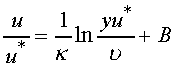 (7)
(7)
where the constants  = 0.41
and B = 5.0. This equation was obtained by examining boundary
layers experimentally. By applying equation (7) at the edged of the
boundary layer where
y = and u =
U, and using the definition of skin-friction coefficient in equation
(4) the following skin-friction law for turbulent flat-plate flow can be
obtained.
= 0.41
and B = 5.0. This equation was obtained by examining boundary
layers experimentally. By applying equation (7) at the edged of the
boundary layer where
y = and u =
U, and using the definition of skin-friction coefficient in equation
(4) the following skin-friction law for turbulent flat-plate flow can be
obtained.
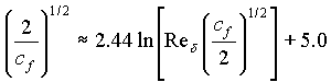 (8)
(8)
Experimental Apparatus
A flat plate with a length of 14 inches has been secured inside
the test section of the AERO lab wind tunnel. A pitot tube is mounted
above the test section (O.D. = 0.10 in) at a distance of approximately
12 inches from the leading edge of the plate. The pitot tube can be moved
in the y-direction above the plate using a traversing mechanism that is scaled
in 0.001" increments (1 revolution = 0.025 in). Both the static and stagnation
pressure taps on the pitot tube are connected to a manometer in order that
the difference between these two pressures may be measured directly in inches
of water. Other instrumentation includes a thermistor inserted into the flow
stream at one of the ports on the side walls of the test section. The air
velocity can be determined from the pressure difference data and the air
density. The wall shear stress and skin-friction coefficent can be calculated
from the velocity profile.
Pitot Tube
If Red > 1000, where d is the probe diameter, the
flow around the probe is nearly frictionless and Bernoulli's equation applies
with good accuracy. For incompressible flow, and neglecting any elevation
head, the following expression relates the local velocity to the difference
in stagnation and static pressure:
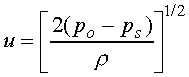 (9)
(9)
where po = stagnation pressure,
ps = static pressure,
and  =
fluid density.
=
fluid density.
The difference between the stagnation and the static pressure can be measured
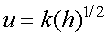
in terms of h inches of water so that equation 9 can be rewritten as
 (10)
(10)
where k is a constant.
Objectives
-
To measure and plot the velocity profile.
-
To compare the free stream velocity to that measured by the wind tunnel
instrumentation.
-
To calculate the wall shear stress and skin friction coefficient.
Procedure
-
Determine the room temperature and the barometric pressure.
-
Set the pitot tube at a reference position at the surface of the plate and
measure the distance from its tip to the leading edge.
-
Zero the wind speed indicator on the AERO lab wind tunnel. Be sure
to start from a positive indication and decrease until it is zeroed.
-
Increase the fan speed of the wind tunnel until a velocity as specified by
the lab assistant is attained.
-
Move the pitot tube at suitable intervals and record the pressure difference
(po - ps) in the manometer and
the reading on the traversing mechanism at each interval. Try to obtain at
least 10 data points within the boundary layer.
Data Reduction & Points of Interest
-
Calculate the free stream velocity in the wind tunnel along with its uncertainty
from the pitot tube measurement. Compare the pitot tube measurement of the
velocity with that obtained from the AERO lab wind tunnel indicator.
Discuss possible reasons for any discrepancies.
-
Calculate the velocity at different y positions and plot the velocity profile
for the experimental data. Compare and discuss this velocity profile to the
expected velocity profile predicted by theory (Blassius solution for laminar
flow or eqtn 7 for turbulent flow).
-
Compute the skin-friction coefficient and wall shear stress and compare to
values predicted from theory. Discuss any differences.
References
-
White, F.M., Fluid Mechanics, 3rd Ed., McGraw-Hill Book Co., New York,
1994.
-
Holman, J.P., Experimental Methods for Engineers, 4th Ed., McGraw-Hill Book
Co., New York, 1984.