BIEN 435 Laboratory

Simulation of Cardiac Output Measurement

Null Hypothesis

This laboratory will be designed to simulate the measurement of cardiac output by the Fick principle. See the accompanying description of the Fick principle. The null hypotheses you would like to test are:

1. The measured value of cardiac output does not depend on the time of injection of the test fluid.
2. The measured value of cardiac output does not depend on the total amount of fluid injected.

In addition, you will compare the signal that you obtain in the “aorta” to the derived relationship of concentration (temperature) as a function of time.

Theory

There are two parts to the theoretical development. The first is the determination of concentration at the detector as a function of time. This has been provided in the handout on the thermal dilution method (Download MS Word File). The second part is the determination of flow rate from the measured concentration.

Consider the situation in Figure 1. Blood is injected into a mixing chamber along with a dye. The concentration is measured at the outlet (Blood + Dye Out). Conservation of mass says that the total mass in must be the total mass out. Total mass in is the concentration in the syringe multiplied by the total volume injected (c_in V). Total mass out is the integral of concentration times flow rate over time. Therefore:

Assume that the flow rate out is constant with time. This is a reasonable assumption as long as the amount of fluid injected is small. Then can be taken out of the integral and the equation can be solved for to yield.

Here, will be known because you know the number of drops per unit volume in the injection syringe. is just the amount of fluid you inject. The integral in the bottom must be obtained from the trace that you will get on the oscilloscope (the output of your concentration detection device). You must find a reasonable way of integrating this trace. One way is to pick values off of the oscilloscope, fit these to the theoretical curve of concentration as a function of time, and then integrate the theoretical curve. Another simple method is to trace the curve on a piece of semitransparent paper, cut out the area under the curve, and weigh the cut out. You can also simply do a Simpson’s rule type of integration, again, from the numbers you pick off the oscilloscope. Whatever method you pick, you must use your calibration curve for concentration to determine concentration from the voltage values and then use this to determine .

Experimental Setup

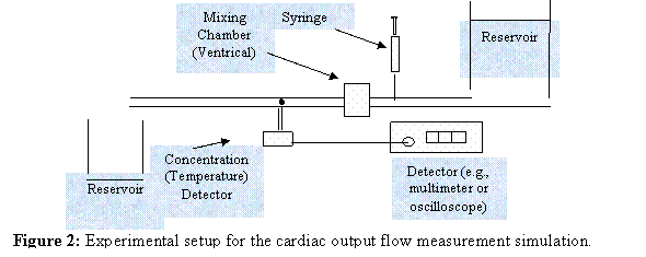
In this experiment you will assemble your own experimental system. Schematically, the system will look like the diagram below: However, it will be up to you to put this system together. Some of the pieces are simple, given what you have done already. Certainly, the two reservoirs and the tubing are already available. You will need to add something to make sure that the injected dye (or hot/cold water) is mixed thoroughly with the flowing water. The concentration detection system can be easily made from a laser, a photoresistor, a voltage supply and a second resistor. You cannot use the digital mutimeter to take readings as a function of time because the concentration will change too quickly to capture. Thus, you will need to use an oscilloscope.

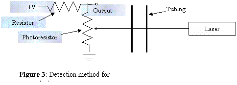
Figure 3 shows a simple concentration detector circuit. The photoresistor changes its resistance according to the amount of light incident on its sensor. As the dye passes in front of the laser, it attenuates the light, causing less light to impinge on the photoresistor. The resistor and the photoresistor form a simple voltage divider so that the output is:

where is the resistance of the photoresistor, is the resistance of the resistor, and is the dc voltage supplied to the circuit. Increased light casues decreased photoresistor voltage, causing reduced output voltage. Since an increased concentration will decrease the amount of light, output voltage increases with concentration.

Transducer Calibration

You will need to calibrate your detector. This should be done in a manner similar to the way you calibrated the pressure transducer in the previous experiment. Should the output be linear, based on the circuit design? I is clear from Eq. 3 that the circuit itself is inherently nonlinear with respect to , but if this nonlinearity can be minimized. Nonetheless, the resistance may still be nonlinear with respect to the amount of light impinging on the photoresistor.

To obtain the calibration, perform a linear least squares fit of concentration as a function of voltage out. This will enable you to translate all of the voltage readings directly to concentration.

Remember to measure the true diameter of the tubing used in this experiment.

Flow Rate

As in the pressure drop experiment, determine the true flow rate. Use a graduated cylinder to set the flow rate to approximately this value. Measure the flow rate as precisely as possible.

Experimental Procedure

To test the two null hypotheses, you will need to measure concentration as a function of time for three cases: 1) Standard amount of injectate over a standard amount of time. 2) Twice the amount of injectate in the same amount of time. 3) Standard amount of injectate over twice the time. You will need at least 5 repetitions for each case to perform your t-test. You will need to use the storage and single sweep trigger features of your oscilloscope.

Data analysis

1. Determine the calibration of your sensor (concentration as a function of voltage).

2. For each data set value of (Volume Collected, Time of Collection), translate to flow rate (Q)

3. Determine a reasonable way to get flow rate from the concentration measurements. This will most likely involve integrating the signal on the oscilloscope in some way.

4. Plot concentration as a function of time.

5. Plot the theoretical curve, based on the experimental values used.

6. Discuss reasons for any differences (theory vs experiment).

7. Perform Student’s T-tests to test the two hypotheses. Provide a p-value in both cases. Are the results significant?